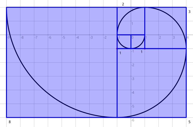
Figure 1. Fibonacci spiral built with the first
6 terms of the sequence.
|
Abstract
The Fibonacci spiral is based on the Fibonacci
sequence to construct a curve forming a spiral. This spiral and
some variants appear in the constructions of live entities. In
this article we present a computed, interactive version of this
spiral
1. The resulting curve can be interactively deformed by
the user while maintaining its internal constraints.
Leonardo Fibonacci, Italian merchandiser, book keeper, mathematician from the XIIIe century, is well known for his Fibonacci sequence, whose terms are called Fibonacci numbers. He made far more mathematical contributions than this sole sequence. He introduced in Europe the Arab digits and its positional system to construct our contemporary numbers, he wrote several treaties on mathematics and accounting.
The Fibonacci sequence is defined by two initial terms and a recurrence relation:
The first few numbers of the sequence are therefore 1, 1, 2, 3, 5, 8.
The Fibonacci spiral is built by using the terms of the sequence as side lengths of squares and by drawing inside each square an inscribed arc of a circle – part of the spiral – whose center lies at one summit of the square and whose radius equals to the square's side length:
|
Figure 1. Fibonacci spiral built with the first
6 terms of the sequence.
|
The construction logic is easy to understand: each square aligns well with its two ancestors according to the recurrence relation. The challenge is how to translate this logic into an iterative process with code in an interactive geometry software. This article presents the steps involved in constructing this programming code.
As the Fibonacci sequence first defines its two first terms, let's look at the first two squares and arcs:
We set two points
Let A be a summit of the first square with
and let M be another summit as well as the center of the arc. The
point A is considered as its origin. To construct the arc we
just need its extremities E=r(A) with the
rotation r
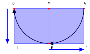 |
Concerning the second square, with , M is still the center of the arc inscribed. The point E becomes its origin. The arc extremity B is built with the same rotation r applied to E, B=r(E). The fourth square summit is built by applying the translation vector to point B
Let's summarize these constructions:
It builds the extremity of the arc when knowing its origin. Its center is the arc center, the angle -90 degrees.
It builds the fourth square summit. Its origin is the arc center, its extremity the arc origin.
The extremity of the first arc becomes the origin of the next one, the center is unchanged.
We translate this description into Dr. Geo code:
|canvas shape alpha a b m s|
canvas := DrGeoCanvas new fullscreen.
alpha := canvas freeValue: -90 degreesToRadians.
shape := [:c :o :f| | e p |
   "c,o,e: center, origin and extremity of the arc"
   e := canvas rotate: o center: c angle: alpha.
   canvas arcCenter: c from: o to: e.
   p := canvas translate: e vector: (canvas vector: c to: o).
   (canvas polygon: { c. o. p. e }) name: f.
   e].
a := canvas point: 1@0.
b := canvas point: -1 @0.
m := canvas middleOf: a and: b.
s := shape value: m value: a value: 1.
shape value: m value: s value: 1.
A few comments:
alpha r the rotation angle is converted into
radian for use in Dr. Geo.
The block of code shape constructs an arc and its
associated square given the center, arc origin and Fibonacci number,
in that order. The block of code returns the arc extremity which is
also the origin of the next arc.
The last two lines show how the extremity s of the first arc is used as the origin of the second arc. The center m remains unchanged.
As the first two terms of the sequence, these two first portions of the spiral are special: same center and radius. In the next section, we adapt this procedure to the remaining part of the spiral.
The third portion spiral has a radius of 2. It is obvious that a change of scale is needed with a homothety:
In this part of the spiral, , we need its center and origin: they are the points A and B. Our block of code shape builds its arc and associated square.
The point E returned as an answer by block shape is also the origin of the next arc, .
The radius of this arc will change from 2 to 3 compared to the previous one, therefore a dilatation of . Then its center is h(A) with the homothety h(E,).
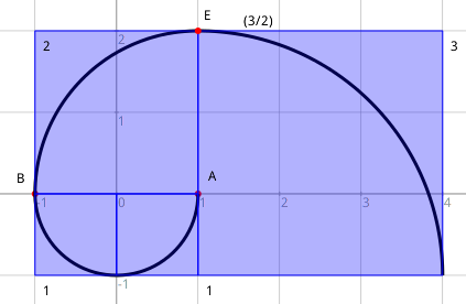 |
Let's summarize these steps:
A spiral portion is built knowing its center A and origin B, the method described in the previous section is used.
The construction above gives the origin E of the next arc. Its center is determined as the transformation of the previous center A with the homothety of center E and the scale . Then the construction step is repeated for the next arc and so on.
We translate this description into the recursive block of code fibo:
fibo := [ :f :o :c :k | | e f1 f2 f3|
"f1: term Fn, f2: term Fn+1,
o & c: origin and center of the arc
e: extremity of the arc/orgin of the next arc"
   f1 := f first.
   f2 := f second.
   f3 := f1 + f2.
   e := shape value: c value: o value: f2.
   c := canvas scale: c center: e factor: f3 / f2.
   k > 0 ifTrue: [
      fibo value: {f2. f3} value: e value: c value: k - 1 ]].
This code deserves a few comments:
The argument f is a list of two terms from the sequence.
k is an iteration counter.
The next iteration occures as long as k > 0, then the block of code is repeated with the arguments: a list with two terms, the origin and center of the next arc and k - 1.
The full code – it can be found in the appendix – is quite short. It comes with the two extracts presented previously. This example illustrates the power of programming; with an appropriate API
2. Application Programming interface
The second interest is to be able to construct a lot of objects, sometime thousands. Finally, the computed sketch is interactive: moving the point A deforms the whole spiral.
 |
So why programming interactive sketches with students? Several themes appear:
Pragmatic use of geometric transformations. Students often question: “What for?” Then of course they can reply: “The spiral, what for?” In its interactive form as we built it, it is a nice example of the interdependent processes met in the mechanical world.
Programming and, with a concise resulting code, its demultiplication power. Young people are not well aware of the programmatic processes surrounding them: “It is tiring to press 50 times the button. Is there a shorter way?” “Yes! But you will have to think harder.”
Resolving a construction problem.
Secondary II students are mathematically equipped to work out this spiral. The recursivity of the block of code matches the recursivity of the Fibonacci sequence and the construction process of the spiral. The programming part required more knowledge, it can be acquired with simpler construction problem. The Dr. Geo' Smalltalk language and environment were designed over the years for kids, indeed from the '70 when computers had strong magical and attractive dimensions, nevertheless the demultiplicating power of programming remains an aspect of strong interest.
|canvas shape alfa fibo a b m s|
canvas := DrGeoCanvas new fullscreen.
alfa := (canvas freeValue: -90 degreesToRadians) hide.
shape := [:c :o :f| | e p |
   e := (canvas rotate: o center: c angle: alfa) hide.
   (canvas arcCenter: c from: o to: e) large.
   p := canvas translate: e vector: (canvas vector: c to: o) hide.
   (canvas polygon: { c. o. p hide. e }) name: f.
   e].
fibo := [ ].
fibo := [ :f :o :c :k | | e f1 f2 f3|
"f1: term Fn-1, f2: term Fn, o & c: origin and center of spiral arm
e: extremity of the spiral arm"
   f1 := f first.
   f2 := f second.
   f3 := f1 + f2.
   e := shape value: c value: o value: f2.
   c := (canvas scale: c center: e factor: f3 / f2) hide.
   k > 0 ifTrue: [
      fibo value: {f2. f3} value: e value: c value: k - 1 ]].
a := canvas point: 1@0.
b := canvas point: -1 @0.
m := (canvas middleOf: a and: b) hide.
s := shape value: m value: a value: 1.
shape value: m value: s value: 1.
fibo value: {1. 2} value: b value: a value: 10